Methodology/Analysis

Many of the data layers collected required minimal processing before being placed into the project folder.  Unless otherwise noted, each layer needed only to be projected to NAD 1983 UTM Zone14N and clipped to the project area of interest (using the county shapefiles taken from TNRIS).

Prioritizing the data allowed for a progressive and discrete set of steps to project completion.  Collection of core data was the focus of each team member, with less emphasis on B and C data layers.  Once the core data had been collected, it was processed, analyzed, and transferred into a Manifold map.  As each non-core data layer was completed, it was subsequently added to the Manifold map.  When time became a factor, we were able to disregard remaining missing or incomplete layers, since they were of the lowest priority. 

Although the bulk of the project consisted of data collection and conversion into an interactive Web interface, there was some analysis of the data required to generate the final data layers, particularly those which were components of the groundwater vulnerability model.  Also, most of the shapefiles obtained from TNRIS were at the quadrangle level of granularity, and there are approximately 325 quadrangles which intersect the Hill Country.  All of these files had to be individually downloaded and unzipped, merged or mosaicked into a single large file, and then clipped to the Hill Country borders. 

Topography and Slope

Surface topography across the region was created by merging contour shapefiles for all 325 quadrangles, then clipping them to the extent of the HCA region.

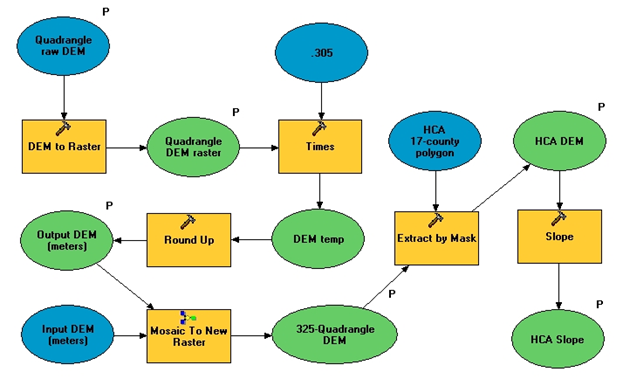
To create a slope layer for the region, the Digital Elevation Model (DEM) files for all 325 quads had to be converted to raster format, transformed to a common scale in meter units of elevation (some DEM files were originally in feet), and mosaicked into a single raster.  This raster was then extracted by mask to the HCA area, and a slope analysis performed, using percentage slope (Figure 3).  The final layer was categorized into 10 classifications each covering a 5% range.

Figure 3. Workflow to produce the final Slope raster

Soil

The raw data consisted of shapefiles (spatial data for primary soil horizons only) plus attribute data derived by running database reports against each county’s data.  Three sets of counties were combined (Blanco + Burnet, Comal + Hays, Edwards + Real), yielding 14 datasets that needed to be processed[1]. 

 The six attributes that were eventually determined to be relevant to the groundwater vulnerability model (GVM) were generated by the Chemical (Calcium Carbonate, Sodium Adsorption Ratio) and Physical (Ksat, Clay %, Linear Extensibility, Organic Matter %) reports. 

After each county’s data were loaded into the primary database, the two reports above were run against each dataset, generating 28 reports.  Each report was then exported into comma-delimited format for further processing in Excel.

In Excel, each report was processed via Text-to-Columns (all data was in the first column) and then prepended with an apostrophe (to enforce text-only data; otherwise some of the range data were automatically translated into calendar dates upon saving).

A repository database was created, and a Visual Basic (VB) program was written to process the 28 files.  The output from the processing for each report was a new table with existing attributes transferred into proper record-field format, plus additional Index (value) fields computed from the six primary GVM attributes.  The VB program exhibited the following assumptions about the data and the computed indices:

1.      For each soil type (the primary key and the spatial key), the record processed was the top/surface layer of the first listed subtype. 

    •          The exception to this rule was that if there was more than one subtype, and the first listed subtype was one of the following [Riverwash, Rock Outcrop, Badlands], then the first subtype was bypassed and the second subtype was processed.

2.      The Index fields created a single value for their respective attributes, which were often expressed as a range in the raw data.  The primary imperative here was to pull the most conservative possible values (those correlating with the greatest vulnerability) which simultaneously created the greatest distinction among different ranges.

•         For attributes where high values correlate with greater vulnerability (Ksat, Linear Extensibility), the highest value in the range was used.

•     For attributes where low values correlate with greater vulnerability (CaCO3, Sodium Adsorption, Organic %, Clay %), the value used was the arithmetic mean of the high and low values in the range.  This allowed for separation both between values reported simply as 0 and those whose lowest range value was 0, and among those with ranges whose lowest value was 0 but whose highest value differed significantly.

Each of these 28 tables was added to ArcGIS along with the 14 spatial datasets provided.  A join was then performed between the spatial dataset and the pair of associated tables, using soil type as the key.  The joined data were exported and trimmed into a county (or multi-county) shapefile, and then all 14 shapefiles were merged into one large 17-county shapefile.

The next general step was to transform the shapefile into a set of six attribute-based raster datasets.  However, because the attributes were text-based, and the raster datasets needed to be number-based, new fields had to be added to the shapefile to hold the numerical data.  As part of this conversion, missing data (represented as “---”) were translated to a value of -1.

Six raster datasets were then created based on the numerical fields, with a resolution (grid size) of 500 meters.  Each raster’s symbology was categorized into seven value ranges, with the  -1 values (representing No Data) in their own category.  The exception was the raster based on Linear Extensibility, which was classified into only five categories due to the limited range of values.  These classifications are detailed in Soil Attribute Reclassification Schemes A & B (Tables 1 and 2) below.

The ultimate output of this process was to be a single composite raster that summed up a given location’s vulnerability across all six attributes.  Each attribute would be given equal weight in this model, which meant that a simple average of the six attribute values would suffice.

Because the actual data values among the rasters were non-comparable, a reference scale was needed.  For ease of computation, a scale of 0-100 was selected, with 100 representing the greatest degree of groundwater vulnerability and 0 the least.  This required a new set of rasters representing this reclassification of values.

For the rasters whose high values corresponded to greater vulnerability, the reclassification was a direct translation of the six categories to values of 0-20-40-60-80-100.  For the others, the classification was similar but inverted (the highest value category was reclassified to 0, and vice versa).  For Linear Extensibility, the new classification was an inverted 0-33-67-100.

In all cases, the value -1 (No Data) was reclassified to 1000.  Had these cells been left as NoData, then every cell that had at least one attribute with NoData would have yielded an output of NoData, thereby ignoring all valid attributes measured at that location.  By setting these cells to a value higher than the maximum possible sum of "real-value" cells (600), it would be apparent in the resultant raster not only which cells had at least one NoData value, but exactly how many each cell had.

The preceding series of steps is depicted in Figure 4.

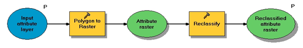
Figure 4.  Conversion from categorized polygon to reclassified raster

The raster calculator was used to perform a direct sum on the six input rasters.  The output was set to show all unique values, and then a final manual reclassification was done whereby all cells with zero NoData values were divided by six, those with one NoData value (i.e., their output value was 1000-1500) were divided by five after subtracting 1000, and so forth.  The final reclassification yielded a composite groundwater vulnerability raster scaled from 0-100 which reflected the relative vulnerability of a given location based on the available data for that location.

Table 1. Soil Attribute Reclassification Scheme A

Table 2. Soil Attribute Reclassification Scheme B

Streamflow Gain/Loss

A study (Slade et. al, 2002) analyzed numerous stream monitoring stations on rivers and streams in the Hill Country.  Several studies were performed along a stream computing the gain flow or loss at each station relative to the nearest upstream station.  These studies were based on readings obtained over a number of years, and can best be explained in the original abstract:

Data for all 366 known stream flow gain-loss studies conducted by the U.S. Geological Survey in Texas were aggregated. A water-budget equation that includes discharges for main channels, tributaries, return flows, and withdrawals was used to document the channel gain or loss for each of 2,872 sub reaches for the studies. The channel gain or loss represents discharge from or recharge to aquifers crossed by the streams. Where applicable, the major or minor aquifer outcrop traversed by each sub reach was identified, as was the length and location for each sub reach. This data will be used to estimate recharge or discharge for major and minor aquifers in Texas, as needed by the Ground-Water Availability Modeling Program being conducted by the Texas Water Development Board. The data also can be used, along with current flow rates for stream flow-gauging stations, to estimate stream flow at sites remote from gauging stations, including sites where stream flow availability is needed for permitted withdrawals (Slade et. Al, 2002, page 1).

The data and results from these studies were provided by the author, and consisted of two separate tables:  1) monitoring station data, including latitude/longitude coordinates, and 2) streamflow studies associated with each station, including gain/loss data.  These tables needed some cleaning up and scrubbing, and the studies needed to be summarized to produce a clean relationship between each station and the streamflow studies associated with that station.  The latitude/longitude coordinates were initially in degrees-minutes-seconds, and had to be converted to decimal degrees.  These updated coordinates were then used to locate each of the monitoring stations.  Finally the average streamflow gain/loss data was categorized to help visually depict the gain or loss at each station.

Internet Mapping Service

An Internet Map Service allows the user to export data from a GIS program into a website accessible by the public.  A tutorial on how to create an IMS is available in the Manifold Users’ Manual www.manifold.net.  In the simplest terms, a user exports a completed Manifold map to a root directory, and then you can publish your map from there.

                                                                                                                                   Go back to aquaKESKA's website!